Plotting Earth relief

PyGMT provides the pygmt.datasets.load_earth_relief function to download the Earth relief data from the GMT remote server and load as an xarray.DataArray object. The data can then be plotted using the pygmt.Figure.grdimage method.

import pygmt

Load sample Earth relief data for the entire globe at a resolution of 1 arc-degree. Refer to pygmt.datasets.load_earth_relief for the other available resolutions.

grid = pygmt.datasets.load_earth_relief(resolution="01d")

gmtread [NOTICE]: Remote data courtesy of GMT data server oceania [http://oceania.generic-mapping-tools.org]
gmtread [NOTICE]: SRTM15 Earth Relief v2.7 at 1x1 arc degrees reduced by Gaussian Cartesian filtering (314.5 km fullwidth) [Tozer et al., 2019].
gmtread [NOTICE]:   -> Download grid file [112K]: earth_relief_01d_g.grd

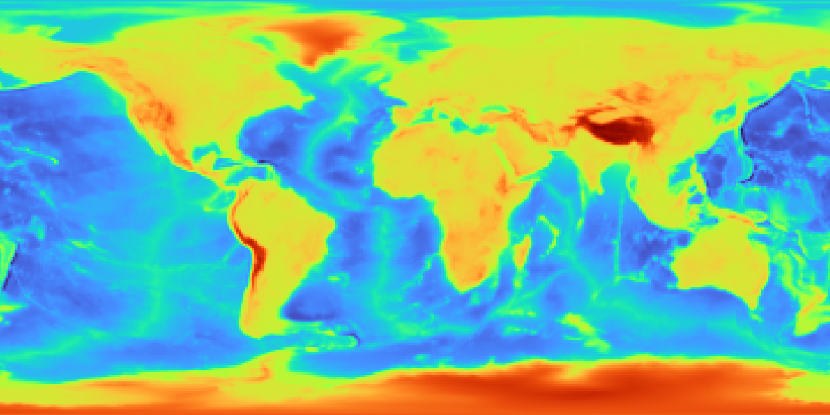
Create a plot

The pygmt.Figure.grdimage method takes the grid input to create a figure. It creates and applies a color palette to the figure based upon the z-values of the data. By default, it plots the map with the turbo CPT, an equidistant cylindrical projection, and with no frame.

fig = pygmt.Figure()
fig.grdimage(grid=grid)
fig.show()

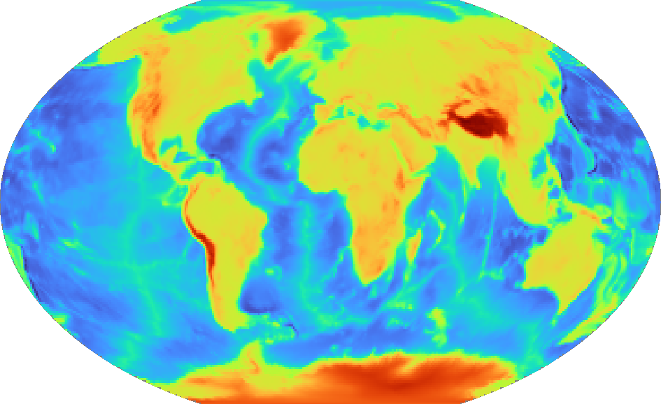
pygmt.Figure.grdimage can take the optional parameter projection for the map. In the example below, projection is set to "R12c" for a 12-centimeters-wide figure with a Winkel Tripel projection. For a list of available projections, see GMT Map Projections.

fig = pygmt.Figure()
fig.grdimage(grid=grid, projection="R12c")
fig.show()

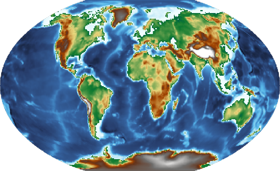
Set a color map

pygmt.Figure.grdimage takes the cmap parameter to set the CPT of the figure. Examples of common CPTs for Earth relief are shown below. A full list of CPTs can be found at https://docs.generic-mapping-tools.org/6.5/reference/cpts.html.

Using the geo CPT:

fig = pygmt.Figure()
fig.grdimage(grid=grid, projection="R12c", cmap="geo")
fig.show()

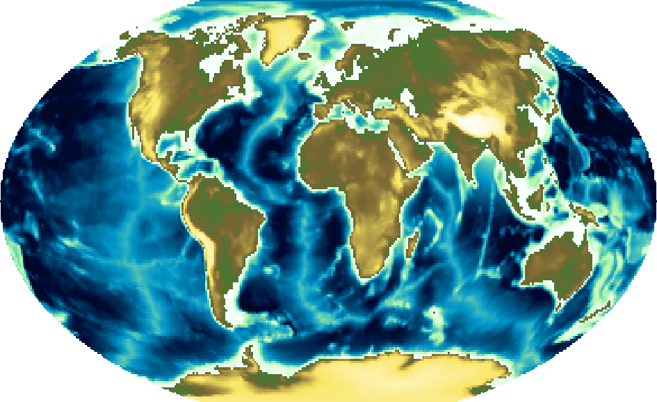
Using the relief CPT:

fig = pygmt.Figure()
fig.grdimage(grid=grid, projection="R12c", cmap="relief")
fig.show()

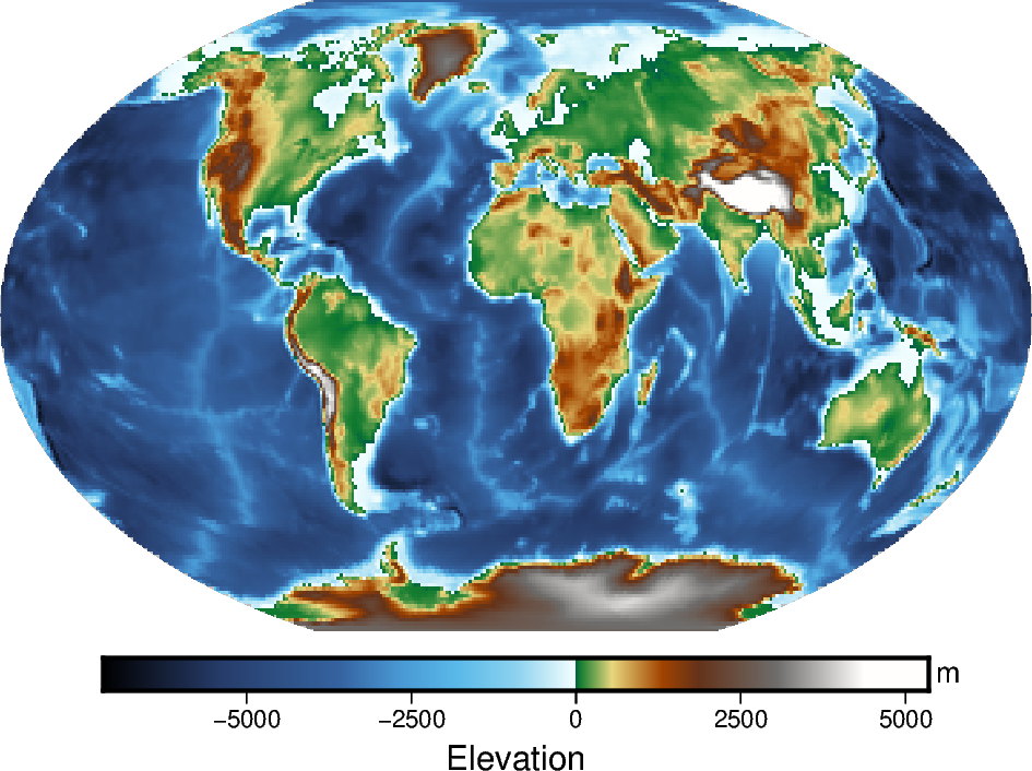
Add a color bar

The pygmt.Figure.colorbar method displays the CPT and the associated z-values of the figure, and by default uses the same CPT set by the cmap parameter for pygmt.Figure.grdimage. The frame parameter for pygmt.Figure.colorbar can be used to set the axis intervals and labels. A list is used to pass multiple arguments to frame. In the example below, "a2500" sets the axis interval to 2,500, "x+lElevation" sets the x-axis label, and "y+lm" sets the y-axis label.

fig = pygmt.Figure()
fig.grdimage(grid=grid, projection="R12c", cmap="geo")
fig.colorbar(frame=["a2500", "x+lElevation", "y+lm"])
fig.show()

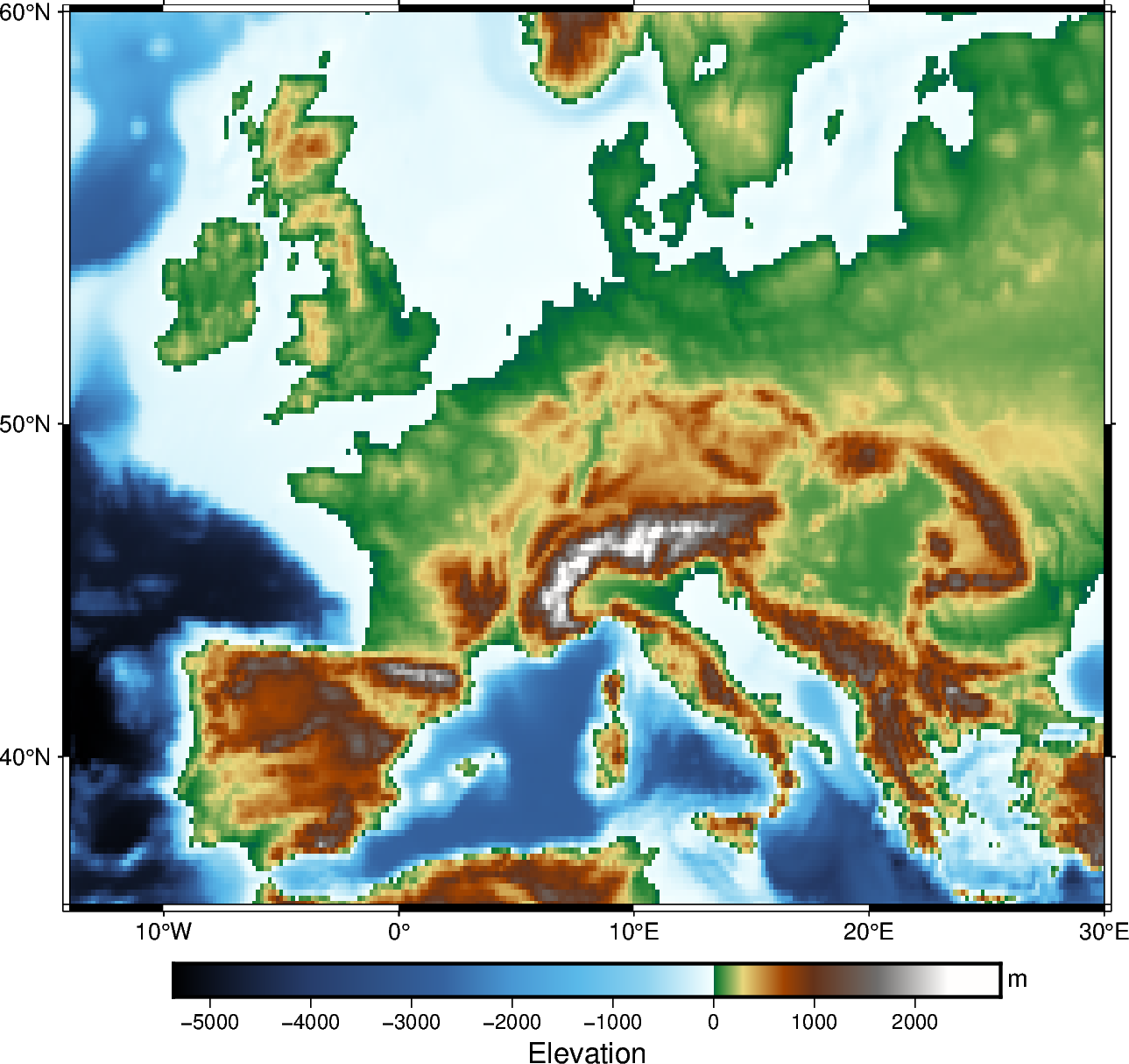
Create a region map

In addition to providing global data, the region parameter of pygmt.datasets.load_earth_relief can be used to provide data for a specific area. The region parameter is required for resolutions at 5 arc-minutes or higher, and accepts a list in the form of [xmin, xmax, ymin, ymax].

The example below uses data with a 10 arc-minutes resolution, and plots it on a 15-centimeters-wide figure with a Mercator projection and a CPT set to geo. frame="a" is used to add a frame with annotations to the figure.

grid = pygmt.datasets.load_earth_relief(resolution="10m", region=[-14, 30, 35, 60])
fig = pygmt.Figure()
fig.grdimage(grid=grid, projection="M15c", frame="a", cmap="geo")
fig.colorbar(frame=["a1000", "x+lElevation", "y+lm"])
fig.show()