Plotting focal mechanisms

Focal mechanisms can be plotted as beachballs with the pygmt.Figure.meca method.

The focal mechanism data or parameters can be provided as various input types: ASCII file, numpy.array, dictionary, or pandas.Dataframe. Different conventions to define the focal mechanism are supported: Aki and Richards ("aki"), global CMT ("gcmt"), moment tensor ("mt"), partial focal mechanism ("partial"), and, principal axis ("principal_axis"). Please refer to the table in the documentation of pygmt.Figure.meca regarding how to set up the input data in respect to the chosen input type and convention (i.e., the expected column order, keys, or column names). In this tutorial we focus on how to adjust the display of the beachballs.

import pandas as pd
import pygmt
from pygmt.params import Pattern

# Set up arguments for basemap
region = [-5, 5, -5, 5]
projection = "X10c/4c"
frame = ["af", "+ggray90"]

Setting up the focal mechanism data

We store focal mechanism parameters for two single events in dictionaries using the moment tensor and Aki and Richards conventions:

# moment tensor convention
mt_single = {
    "mrr": 4.71,
    "mtt": 0.0381,
    "mff": -4.74,
    "mrt": 0.399,
    "mrf": -0.805,
    "mtf": -1.23,
    "exponent": 24,
}
# Aki and Richards convention
aki_single = {"strike": 318, "dip": 89, "rake": -179, "magnitude": 7.75}

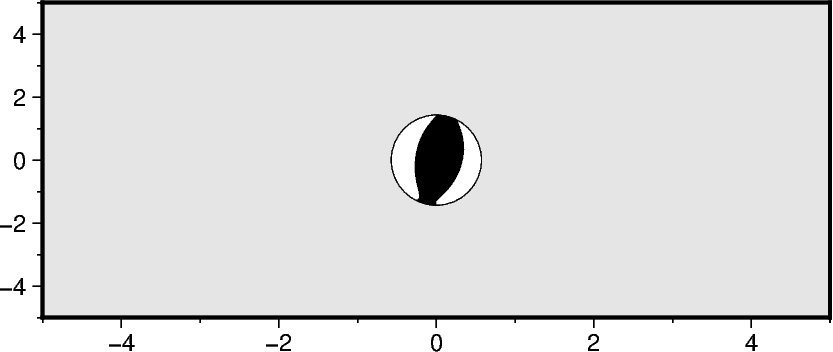
Plotting a single beachball

Required parameters are spec and scale as well as longitude, latitude (event location), and depth (if these values are not included in the argument passed to spec). Additionally, the convention parameter is required if spec is an 1-D or 2-D numpy array; for the input types dictionary and pandas.Dataframe, the focal mechanism convention is automatically determined from dictionary keys or pandas.DataFrame column names. The scale parameter controls the radius of the beachball. By default, the value defines the size for a magnitude of 5 (i.e., a scalar seismic moment of \(M_0 = 4.0 \times 10^{23}\) dyn cm) and the beachball size is proportional to the magnitude. Append "+l" to force the radius to be proportional to the seismic moment.

fig = pygmt.Figure()
fig.basemap(region=region, projection=projection, frame=frame)

fig.meca(spec=mt_single, scale="1c", longitude=0, latitude=0, depth=0)

fig.show()

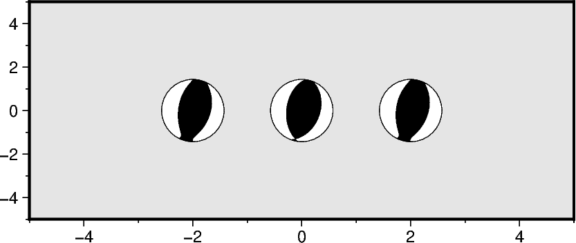
Plotting the components of a seismic moment tensor

A moment tensor can be decomposed into isotropic and deviatoric parts. The deviatoric part can be further decomposed into multiple parts (e.g., a double couple (DC) and a compensated linear vector dipole (CLVD)). Use the component parameter to specify the component you want to plot.

fig = pygmt.Figure()
fig.basemap(region=region, projection=projection, frame=frame)

for component, longitude in zip(["full", "dc", "deviatoric"], [-2, 0, 2], strict=True):
    fig.meca(
        spec=mt_single,
        scale="1c",
        longitude=longitude,
        latitude=0,
        depth=0,
        component=component,
    )

fig.show()

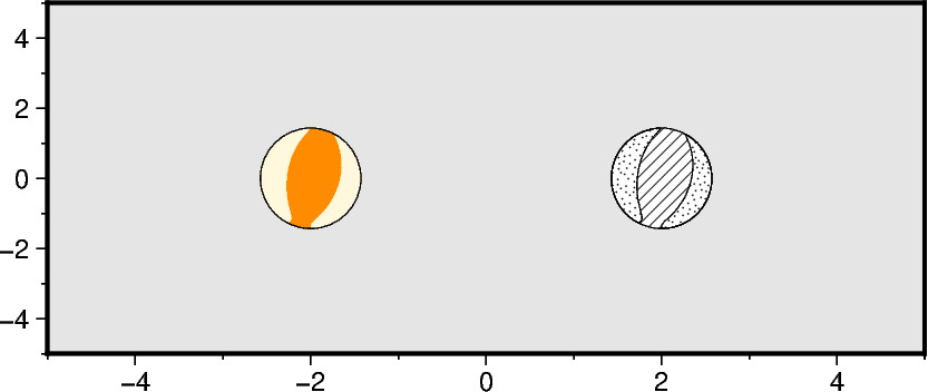
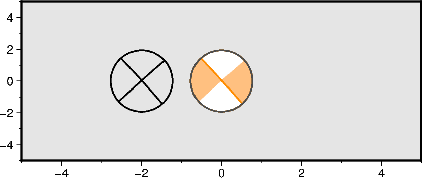
Filling the quadrants

Use the parameters compressionfill and extensionfill to fill the quadrants with different colors or patterns.

fig = pygmt.Figure()
fig.basemap(region=region, projection=projection, frame=frame)

fig.meca(
    spec=mt_single,
    scale="1c",
    longitude=-2,
    latitude=0,
    depth=0,
    compressionfill="darkorange",
    extensionfill="cornsilk",
)

fig.meca(
    spec=mt_single,
    scale="1c",
    longitude=2,
    latitude=0,
    depth=0,
    compressionfill=Pattern(8),
    extensionfill=Pattern(31),
    outline=True,
)

fig.show()

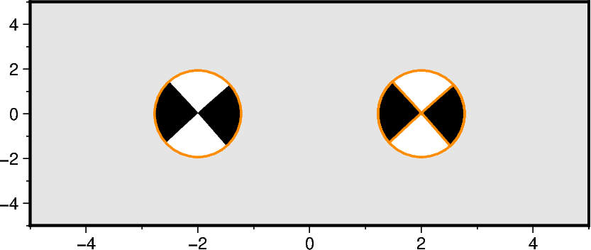
Adjusting the outlines

Use the parameters pen and outline for adjusting the circumference of the beachball or all lines (i.e, circumference and both nodal planes).

fig = pygmt.Figure()
fig.basemap(region=region, projection=projection, frame=frame)

fig.meca(
    spec=aki_single,
    scale="1c",
    longitude=-2,
    latitude=0,
    depth=0,
    # Use a 1-point thick, darkorange and solid line
    pen="1p,darkorange",
)

fig.meca(
    spec=aki_single,
    scale="1c",
    longitude=2,
    latitude=0,
    depth=0,
    outline="1p,darkorange",
)

fig.show()

Highlighting the nodal planes

Use the parameter nodal to highlight specific nodal planes. "0" refers to both, "1" to the first, and "2" to the second nodal plane(s). Only the circumference and the specified nodal plane(s) are plotted, i.e. the quadrants remain unfilled (transparent). We can make use of the stacking concept of (Py)GMT, and use nodal in combination with the outline, compressionfill / extensionfill and pen parameters.

fig = pygmt.Figure()
fig.basemap(region=region, projection=projection, frame=frame)

fig.meca(
    spec=aki_single,
    scale="1c",
    longitude=-2,
    latitude=0,
    depth=0,
    nodal="0/1p,black",
)

# Plot the same beachball three times with different settings:
# (i) Fill the compressive quadrants
# (ii) Plot the first nodal plane and the circumference in darkorange
# (iii) Plot the circumfence in black on top; use "-" to not fill the quadrants
for kwargs in [
    {"compressionfill": "lightorange"},
    {"nodal": "1/1p,darkorange"},
    {"compressionfill": "-", "extensionfill": "-", "pen": "1p,gray30"},
]:
    fig.meca(
        spec=aki_single,
        scale="1c",
        longitude=0,
        latitude=0,
        depth=0,
        **kwargs,
    )
fig.show()

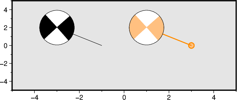
Adding offset from event location

Specify the optional parameters plot_longitude and plot_latitude. If spec is an ASCII file with columns for plot_longitude and plot_latitude, the offset parameter has to be set to True. Besides just drawing a line between the beachball and the event location, a small circle can be plotted at the event location by appending +s and the descired circle diameter. The connecting line as well as the outline of the circle are plotted with the setting of pen, or can be adjusted separately. The fill of the small circle corresponds to the fill of the compressive quadrantes.

fig = pygmt.Figure()
fig.basemap(region=region, projection=projection, frame=frame)

fig.meca(
    spec=aki_single,
    scale="1c",
    longitude=-1,
    latitude=0,
    depth=0,
    plot_longitude=-3,
    plot_latitude=2,
)

fig.meca(
    spec=aki_single,
    scale="1c",
    longitude=3,
    latitude=0,
    depth=0,
    plot_longitude=1,
    plot_latitude=2,
    offset="+p1p,darkorange+s0.25c",
    compressionfill="lightorange",
)

fig.show()

Plotting multiple beachballs

Now we want to plot multiple beachballs with one call of pygmt.Figure.meca. We use data of four earthquakes taken from USGS. For each focal mechanism parameter a list with a length corresponding to the number of events has to be given.

# Set up a pandas.DataFrame with multiple focal mechanism parameters.
aki_multiple = pd.DataFrame(
    {
        "strike": [255, 173, 295, 318],
        "dip": [70, 68, 79, 89],
        "rake": [20, 83, -177, -179],
        "magnitude": [7.0, 5.8, 6.0, 7.8],
        "longitude": [-72.53, -79.61, 69.46, 37.01],
        "latitude": [18.44, 0.90, 33.02, 37.23],
        "depth": [13, 19, 4, 10],
        "plot_longitude": [-70, -110, 100, 0],
        "plot_latitude": [40, 10, 50, 55],
        "event_name": [
            "Haiti - 2010/01/12",
            "Esmeraldas - 2022/03/27",
            "Afghanistan - 2022/06/21",
            "Syria/Turkey - 2023/02/06",
        ],
    }
)

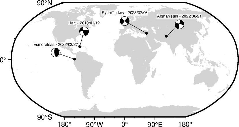
Adding a label

Use the optional parameter event_name to add a label near the beachball, e.g., event name or event date and time. Change the font of the label text by appending +f and the desired font (size,name,color) to the argument passed to the scale parameter. Additionally, the location of the label relative to the beachball [Default is "TC", i.e., Top Center] can be changed by appending +j and an offset can be applied by appending +o with values for dx/dy. Add a colored [Default is white] box behind the label via the label labelbox. Force a fixed size of the beachball by appending +m to the argument passed to the scale parameter.

fig = pygmt.Figure()
fig.coast(region="d", projection="N10c", land="lightgray", frame=True)

fig.meca(spec=aki_multiple, scale="0.4c+m+f5p", labelbox="white@30", offset="+s0.1c")

fig.show()

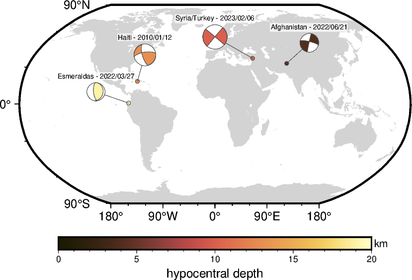
Using size-coding and color-coding

The beachball can be sized and colored by the quantities given as magnitude and depth, e.g., by moment magnitude or hypocentral depth, respectively. Use the parameter cmap to pass the descired colormap. Now, the fills of the small circles indicating the event locations are given by the colormap.

fig = pygmt.Figure()
fig.coast(region="d", projection="N10c", land="lightgray", frame=True)

# Set up colormap and colorbar for hypocentral depth
pygmt.makecpt(cmap="lajolla", series=[0, 20])
fig.colorbar(frame=["x+lhypocentral depth", "y+lkm"])

fig.meca(
    spec=aki_multiple,
    scale="0.4c+f5p",
    offset="0.2p,gray30+s0.1c",
    labelbox="white@30",
    cmap=True,
    outline="0.2p,gray30",
)

fig.show()